3D Ultrasound Enables Accurate, Noninvasive Measurements of Blood Flow
Released: June 30, 2020
At A Glance
- 3D ultrasound provides an effective, noninvasive way to estimate blood flow.
- Measurements of blood flow are important in cases of chronic illnesses and emergency situations.
- The research was the work of Quantitative Imaging Biomarkers Alliance (QIBA).
- RSNA Media Relations
1-630-590-7762
media@rsna.org - Linda Brooks
1-630-590-7738
lbrooks@rsna.org - Dionna Arnold
1-630-590-7791
darnold@rsna.org
OAK BROOK, Ill. — A 3D ultrasound system provides an effective, noninvasive way to estimate blood flow that retains its accuracy across different equipment, operators and facilities, according to a study published in the journal Radiology.
Measures of blood flow are important in helping clinicians determine how much oxygen and nutrient-carrying blood is reaching organs and tissues in a patient’s body. In emergency situations, accurate blood flow measurements can show if there is adequate blood supply to organs like the heart and brain. Blood flow measurements are important in chronic conditions too, as in the cases of measuring blood flow to the feet and lower limbs of people with diabetes.
Despite its importance, there is no ideal way to measure blood flow noninvasively and inexpensively. Current methods like blood pressure and 2D ultrasound (i.e., spectral Doppler) provide only surrogate metrics rather than the desired volumetric flow or have substantial limitations and are prone to errors. True flow measurements with 2D ultrasound are rarely used clinically due to reliability issues and cumbersome implementation. In addition, results often vary considerably between facilities and operators. Measurements from an experienced ultrasound technologist might differ significantly from those of a less experienced one.

“Right now, we just don’t have anything better to quantify blood flow,” said study lead author Oliver D. Kripfgans, Ph.D., associate professor of radiology from the Department of Radiology at Michigan Medicine in Ann Arbor, Michigan.
Dr. Kripfgans and his Michigan Medicine colleagues J. Brian Fowlkes, Ph.D., Stephen Z. Pinter, Ph.D., and Jonathan M. Rubin, M.D., Ph.D., have spent years developing and studying a 3D approach for quantitatively measuring blood flow. For the new study, he and his colleagues, along with other volunteers involved in the Quantitative Imaging Biomarkers Alliance (QIBA), tested this 3D approach on three clinical scanners using a custom flow phantom, a device that mimics blood flow in humans. They used seven different laboratories and manipulated the testing conditions by changing flow rate, imaging depth and other parameters for a total of eight distinct testing conditions.
The results showed that blood volume flow estimated by 3D color-flow ultrasound was accurate and reproducible among the seven laboratories.
“We had less than 10% error or variation,” Dr. Kripfgans said. “For some of the systems, we were down to only 3% to 5% difference between labs. These are fantastic results that show that, from a technology point of view, some systems could be ready to go to the clinic.”
Dr. Kripfgans credited the simplicity of the 3D approach, ease of data collection and elimination of assumptions plaguing other methods for minimizing the variation in results between users and systems. That simplicity, coupled with the availability of 3D on many existing ultrasound systems, is likely to hasten its arrival to clinical medicine, Dr. Kripfgans said.
“Once the technique becomes available commercially on scanners, clinical adoption will be much faster because then it’s not a research project anymore, it’s something that’s readily available, and after that it’s just a matter of time before it reaches the clinic,” he said.
QIBA, an alliance of researchers, health care professionals and industry representatives, was organized by the Radiological Society of North America in 2007 to improve current biomarkers and investigate new ones. Biomarkers are measurable indicators of the state of a person’s health.
The QIBA initiative includes collaboration to identify needs, barriers and solutions to create consistent, reliable, valid and achievable quantitative imaging results across imaging platforms, clinical sites, and time. QIBA aims to accelerate development and adoption of hardware and software standards to achieve accurate and reproducible quantitative results from imaging methods.
“Because of QIBA and this study I’m confident that this 3D ultrasound technology is on a path to the clinic,” Dr. Kripfgans said.
“Three-dimensional US for Quantification of Volumetric Blood Flow: Multisite Multisystem Results from within the Quantitative Imaging Biomarker Alliance.” Collaborating with Drs. Kripfgans, Fowlkes, Pinter and Rubin were Cristel Baiu, M.Sc., Matthew F. Bruce, Ph.D., Paul L. Carson, Ph.D., Shigao Chen, Ph.D., Todd N. Erpelding, Ph.D., Jing Gao, M.D., Mark E. Lockhart, M.D., M.P.H., Andy Milkowski, M.Sc., Nancy Obuchowski, Ph.D., Michelle L. Robbin, M.D., M.S., and James A. Zagzebski, Ph.D.
Radiology is edited by David A. Bluemke, M.D., Ph.D., University of Wisconsin School of Medicine and Public Health, Madison, Wisconsin, and owned and published by the Radiological Society of North America, Inc. (https://pubs.rsna.org/journal/radiology)
RSNA is an association of radiologists, radiation oncologists, medical physicists and related scientists promoting excellence in patient care and health care delivery through education, research and technologic innovation. The Society is based in Oak Brook, Illinois. (RSNA.org)
For patient-friendly information on ultrasound, visit RadiologyInfo.org.
Images (JPG, TIF):
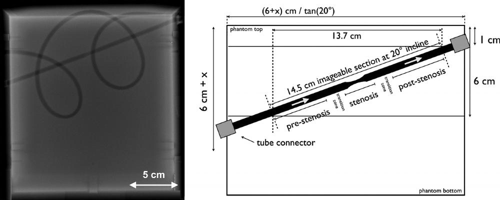
Figure 1. Flow phantom description. Radiograph (left side) shows a linear tube section angled at a 20° incline from left to right. This linear section included a 40% stenosis (ie, a 5- to 3-mm diameter reduction plus subsequent expansion back to 5 mm) over a 3-cm tube length. There is also a curved tubing section that forms two loops. These are intended to be anatomically curved and possess diameter fluctuations with a mean of 5 mm. Schematic (right side) shows the position of stenotic tubing section. Stenotic section and transition zone are not to scale.
High-res (TIF) version
(Right-click and Save As)
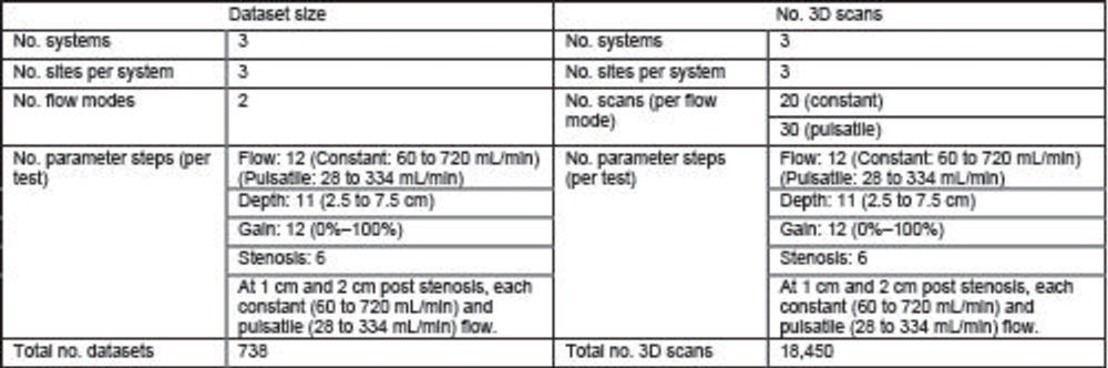
Figure 2. Structure of the multisite multisystem study, with three systems at three different sites per system. The study at each site included four tests (flow, depth, gain, and stenosis) taken under constant and pulsatile flow. This resulted in a total of 738 datasets consisting of 18,450 image volumes. 3D = three-dimensional.
High-res (TIF) version
(Right-click and Save As)
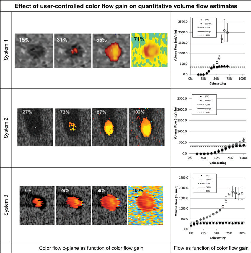
Figure 3. Volume flow as a function of color flow gain (at a single testing site). For each row the color flow c-plane and the computed volume flow are shown as a function of color flow gain. The c-plane is shown for four representative gain levels, whereas the computed volume flow is shown for 12–17 steps across the available gain settings. Flow was computed with (solid circles on the graphs) and without (hollow circles on the graphs) partial volume correction. Partial volume correction accounts for pixels that are only partially inside the lumen. Therefore, high gain (ie, blooming) does not result in overestimation of flow. Systems 1 and 2 converge to true flow after the lumen is filled with color pixel. System 3 is nearly constant regarding gain and underestimates the flow by approximately 17%. Shown are mean flow estimated from 20 volumes, and the error bars show standard deviation.
High-res (TIF) version
(Right-click and Save As)
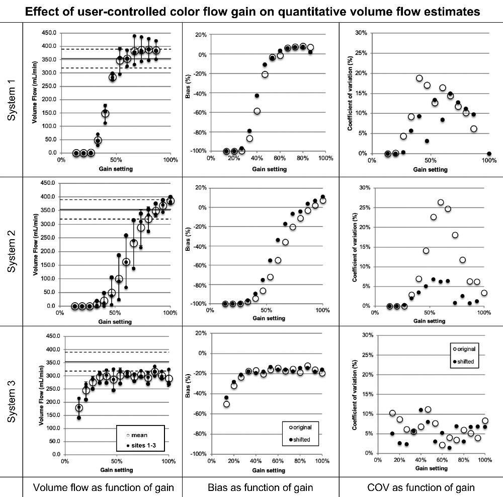
Figure 4. Volume flow as a function of color flow gain. Shown for each row are (left) volume flow (small •) for systems 1, 2, and 3, respectively, and the mean flow (large ⃝) and (middle and right) mean bias and coefficient of variation of mean flow between sites (large ⃝), respectively. Possible differences in system sensitivity between systems 1, 2, and 3 were compensated by allowing a gain offset between sites. The results are shown (small •). System 2 shows a decrease of coefficients of variation from a maximum of greater than 25% before compensation to 7% after compensation (P = .002). Systems 1 and 3 show no appreciable change. COV = coefficient of variation.
High-res (TIF) version
(Right-click and Save As)
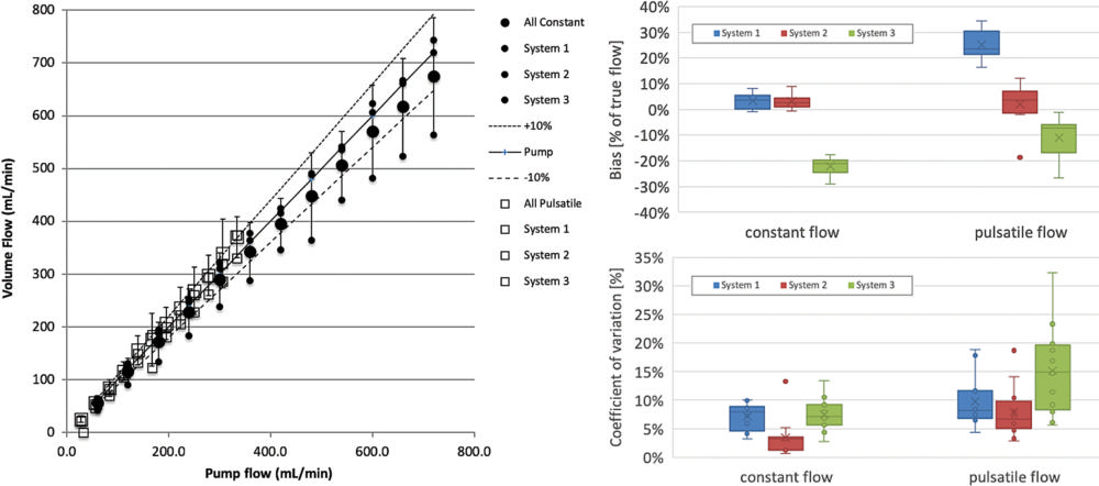
Figure 5. Computed volume flow as a function of pump flow rate shows volume flow versus pump flow rate (left side), bias in percent of true flow (top right side), and coefficient of variation (lower right side). Data shown are from three systems (blue, red, green) averaged across three sites each at two conditions (constant flow and pulsatile flow). The identity of the systems is hidden by using uniform plot symbols. Constant flow (left) is plotted (•). Mean across systems 1, 2, and 3 is shown (large •), which are also shown (small •). Pulsatile flow is plotted (□). The mean (large □) across systems 1, 2, and 3 is shown, and their means are also shown (small □). Box and whisker plots of bias and coefficient of variation for all systems (right side) are shown and split into constant and pulsatile flow. Box plots are shown with error bars (standard deviation), mean (x), median (horizontal line in each box), and 25th–75th percentile range for each system and flow condition. The mean biases (top right) for systems 1, 2, and 3 are, respectively, 3.5%, 3.0%, and –22.1% for constant flow, and 24.9%, 2.1%, and –10.9% for pulsatile flow. Coefficients of variation (bottom right) as box plots for the same data are, respectively, 6.9%, 3.3%, and 9.6% for constant flow and 7.7%, 8.2%, and 17.3% for pulsatile flow.
High-res (TIF) version
(Right-click and Save As)
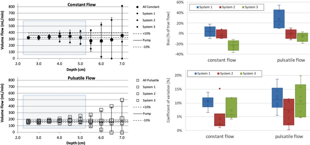
Figure 6. Computed volume flow as a function of c-plane (lateral elevational plane of equal distance from the transducer) depth. The left side shows volume flow versus c-plane depth for constant and pulsatile flow in top and bottom panel, respectively. The right side shows box and whisker plots that show bias for each system averaged across sites in percent of true flow within the blue shaded range in the left-side panel. Coefficient of variation is shown (lower right side) for the same blue shaded range of the left-side panel. Data shown are composed of three systems at two conditions, constant flow and pulsatile flow. Constant flow is plotted (upper left side; •). The mean across systems 1, 2, and 3 is shown (large •), and each system mean is shown (small •). The identity of the systems is hidden by using uniform plot symbols. Pulsatile flow is plotted (lower left; □). The mean across systems 1, 2, and 3 is shown (large □), and each system mean is shown (small □). Box plots of bias (top right) and coefficient of variation (bottom right) for all systems are split into constant and pulsatile flow. Box plots are shown with error bars (standard deviation), mean (x), median (horizontal line), and 25th–75th percentile range for each system and flow condition. The mean biases for systems 1, 2, and 3 are, respectively, 3.7%, –2.0%, and –22.8% for constant flow and 27.2%, –0.9%, and –5.9% for pulsatile flow. The mean coefficients of variation are, respectively, 10.0%, 4.6%, and 10.1% for constant flow and 9.2%, 6.9%, and 11.6% for pulsatile flow.
High-res (TIF) version
(Right-click and Save As)
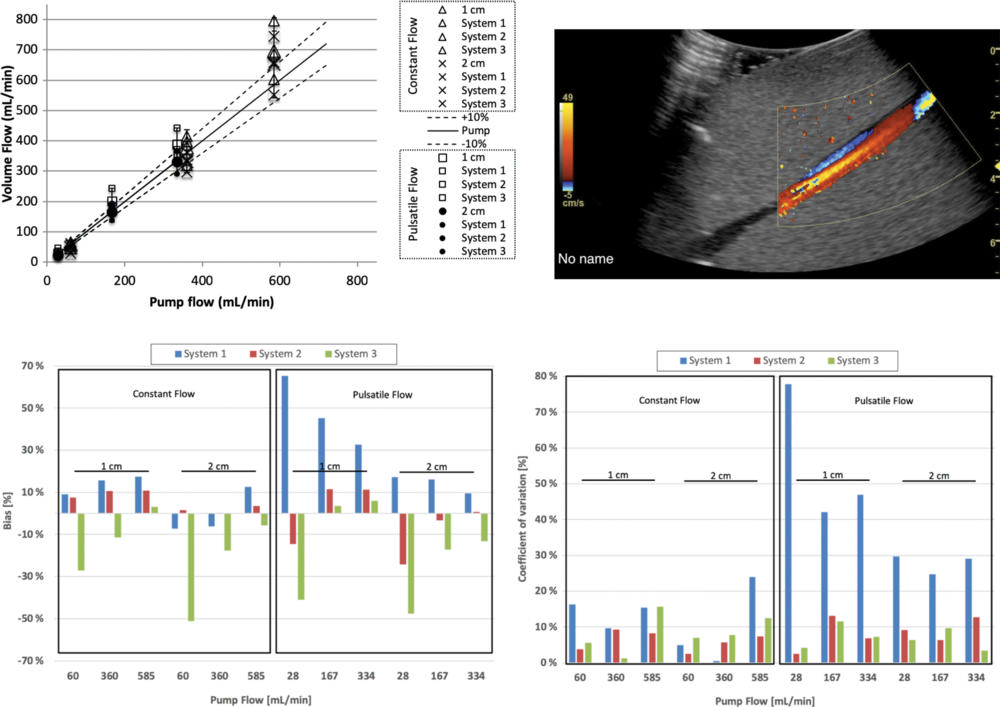
Figure 7. Volume flow computation of flow distal (downstream) to a 40% stenosis. Computed flow at c-planes (ie, the lateral elevational plane of equal distance from the transducer) located 1 and 2 cm past the stenosis at constant and pulsatile flow conditions. Top left graph shows computed volume flow as a function of pump flow. Constant flow is shown at 1 cm (∆) and 2 cm (X) distal (ie, downstream) to the stenosis and pulsatile flow at 1 cm (□) and 2 cm (•) distal (downstream) to the stenosis, respectively. For constant flow, bias and coefficient of variation are almost all less than 20%. Figure 2 shows analysis of these results. Example screenshot (top right) is shown for poststenotic flow. Bias at 1 and 2 cm poststenosis (bottom left) is shown and averaged between three sites. Coefficient of variation at 1 and 2 cm poststenosis (bottom right) is shown and averaged between three sites.
High-res (TIF) version
(Right-click and Save As)